Wednesday: Accuracy, Logistic Regression

Chapter 1: Accuracy

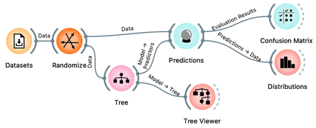
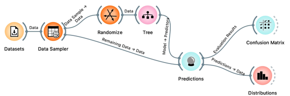
Now that we know what classification trees are, the next question is what is the quality of their predictions. For beginning, we need to define what we mean by quality. In classification, the simplest measure of quality is classification accuracy expressed as the proportion of data instances for which the classifier correctly guessed the value of the class. Let's see if we can estimate, or at least get a feeling for, classification accuracy with the widgets we already know, plus with a new widget that displays so-called confusion matrix.

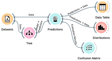
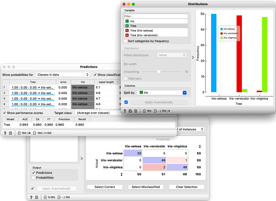
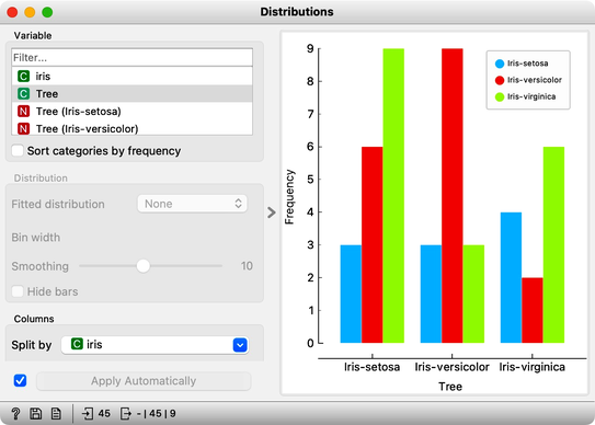
Let us use this workflow with the Iris flower data set. The Predictions widget outputs a data table augmented with a column that includes predictions. In the Data Table widget, we can sort the data by any of these two columns, and manually select data instances where the values of these two features are different (this would not work on big data). Roughly, visually estimating the accuracy of predictions is straightforward in the Distribution widget, if we set the features in the view appropriately. Iris setosas are all classified correctly, and for the other two species there are just three misclassifications. Classification accuracy is thus (150-3)/150 = 0.98, that is, our tree classifier is 98% correct. This same statistics on correctly and incorrectly classified examples is also provided in the Confusion Matrix widget.

Chapter 2: How to Cheat

This lesson has a strange title and it is not obvious why it was chosen. Maybe you, the reader, should tell us what this lesson has to do with cheating.

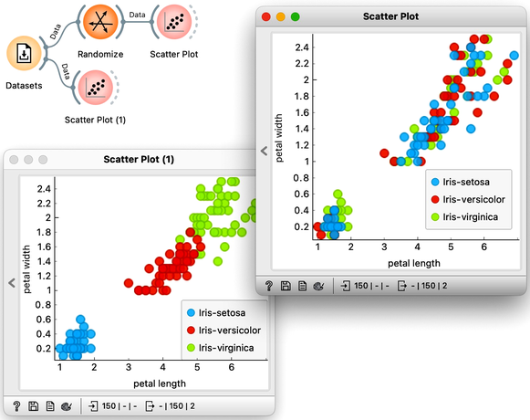
At this stage, the classification tree on the Iris flower data set looks very good. There are only three data instances where the tree makes a mistake. Can we mess up the data set so bad that the trees will ultimately fail? Like, remove any existing correlation between features and the class? We can! There's the Randomize widget with class shuffling. Check out the chaos it creates in the Scatter Plot visualization where there were nice clusters before randomization, and where now, of course, the classes have been messed up.

Scatter plot of the original Iris data set the data set after shuffling the class of 100% of rows.

Fine. There can be no classifier that can model this mess, right? Let us check out if this is indeed so.

And the result? Here is a screenshot of the Distributions widget.

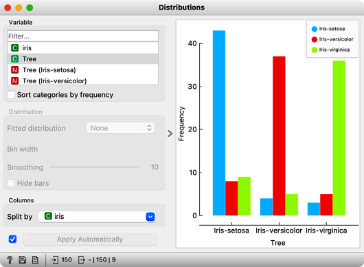
Most unusual. Despite shuffling all the classes, which destroyed any connection between features and the class variable, about 80% of predictions were still correct.

Can we further improve accuracy on the shuffled data? Let us try to change some properties of the induced trees: in the Tree widget, disable all early stopping criteria.

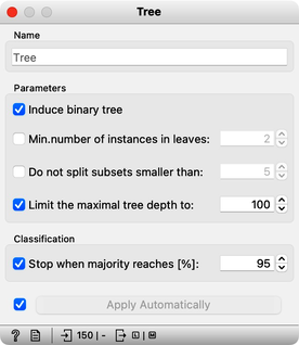
Wow, almost no mistakes now, the accuracy of predictions is nearly 99%. How is this possible? On a class-randomized data set? To find the answer to this riddle, open the Tree Viewer and check out the tree. How many nodes does it have? Are there many data instances in the leaf nodes?

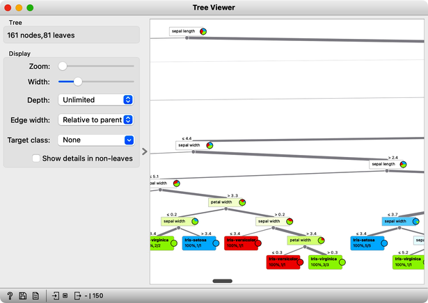
With 161 nodes and 81 leaves the tree is huge and it is impossible to visualize it in a modest-size window. It is perhaps even more complex than the Iris data table itself. Looks like the tree just memorized every data instance from the data set. No wonder the predictions were right. The tree makes no sense, and it is complex because it simply remembered everything.

Ha, if this is so, if a classifier remembers everything from a data set but without discovering any general patterns, it should perform miserably on any new data set. Let us check this out. We will split our data set into two sets, training and testing, randomize the train and feed it into the classification tree and then estimate its accuracy on the test data set.

Notice that we needed to rewire the connection between Data Sampler and Predictions, so that remaining, out-of-sample data is feed to Predictions.

Let’s use the Distributions widget to check how the classifications look like after testing the classifier on the test data.

The results are a complete fail. The tree almost predicts for almost equal frequency that the Iris is setosa, regardless of original, true class. On the class-randomized training data our classifier fails miserably. Finally, just as we would expect.

We have just learned that we need to train the classifiers on the training set and then test it on a separate test set to really measure performance of a classification technique. With this test, we can distinguish between those classifiers that just memorize the training data and those that actually learn a general model.

Learning is not only memorizing. Rather, it is discovering patterns that govern the data and apply to new data as well. To estimate the accuracy of a classifier, we therefore need a separate test set. This estimate should not depend on just one division of the input data set to training and test set (here's a place for cheating as well). Instead, we need to repeat the process of estimation several times, each time on a different train/test set and report on the average score.

Chapter 3: Cross-Validation

So how would the right estimation of the accuracy of the tree classifier look like. In the previous chapter, we have learned that we need to split the data to training and test set, that is, we need to test the model on the data that the model has not seen in the testing phase. Else, it is just as we would always accurately predict yesterday's weather. Let us do so without randomization, and set the tree parameters back so that they enable some forward pruning of the tree.

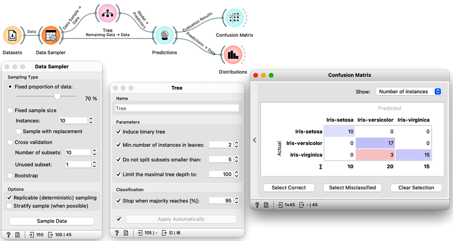
It looks like our classification tree indeed has high estimated accuracy. Only three iris flowers were misclassified. But this estimate can depend on the random split of the data. Let us check this out. In the Data Sampler, we will uncheck replicable sampling, click, perhaps several times, the Sample Data button and observe if there are any changes in the confusion matrix.

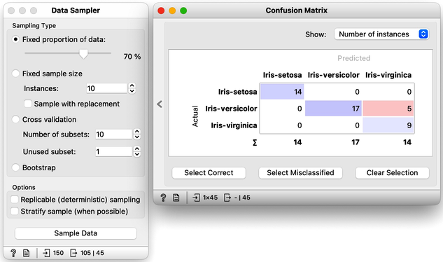
On every click on the Sample Data button, the widget emits the new random sample, and the confusion matrix changes. The number of errors is small, and usually fluctuates between misclassifing versicolor and virginica. If we are really lucky, the composition of the training and test set is such that the tree inferred on the training set makes no errors on the test set.

So if we are about to write a paper on the utility of the machine learning for some data set, which error would we report? The minimal one that we obtain? The maximal one? Actually, none of these. Remember, the split of the data to the training and test set only provides means to estimate the error the tree would make if presented a new data set. A solid estimate would not depend on particular sampling of the data. Therefore, it is best to sample many times, like 100 times, and report on the average accuracy.

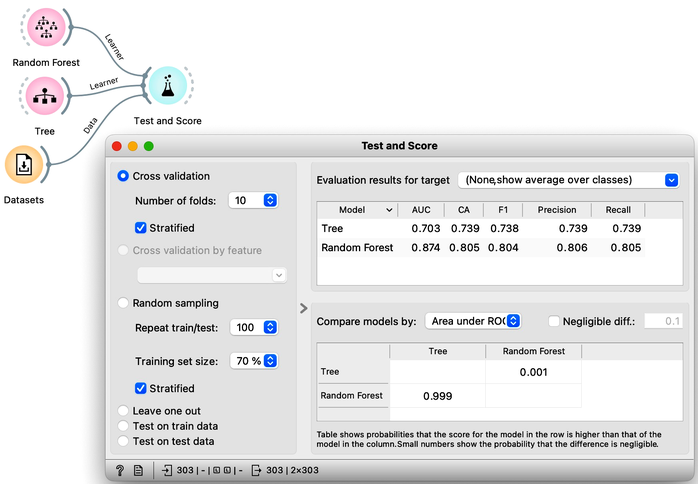
Pressing Sample Data button a hundred times and computing the average score would be really boring. Instead, Orange has a widget that does all that for us. The widget is called Test and Score. To repeat training and testing 100 times with the same training algorithm, we have to provide it a data set and the training algorithm. The widget then iteratively splits the data, uses the training algorithm to develop a predictive model on the subset of data for training, uses the resulting model on the test data and calculates the accuracy, and at the end reports an average accuracy (column called "CA") from all the iterations.

The Test and Score uses the training algorithm, not a model. Hence, the Tree widget sends it the Learner, an object storing a learning method. Why is there no connection needed between the Datasets and the Tree?

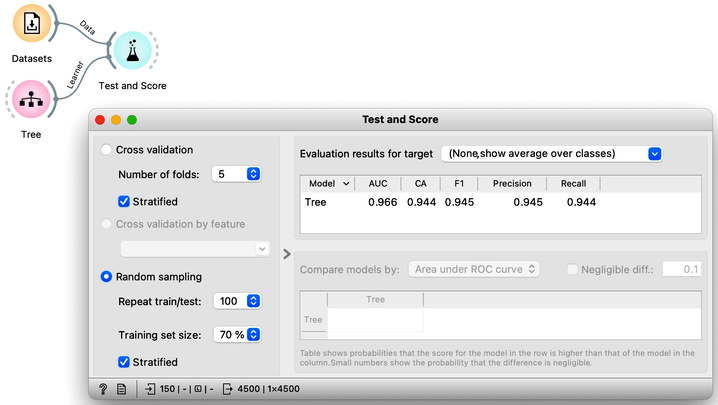
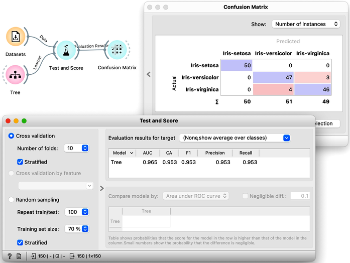
While we could conclude our discussion at this point, there is an alternative and more widely-used method for estimating accuracy that we should consider. This method, called cross-validation, avoids the possibility that certain data instances will be placed into the test set more frequently than others by randomly splitting the data multiple times. Instead, each data instance is included in the test set exactly once. To perform cross-validation, the data is first divided into k folds. Then, in each of the k iterations, one fold is used for testing while the remaining folds are used for training. Typically, k is set to 10, but in Orange, the default value of 5 is used to conserve computing resources. The results of performing ten-fold cross-validation on the Iris flower data set are shown below. To ensure that each fold contains a roughly equal distribution of classes, the "stratification" option is utilized during the creation of the folds.

Another advantage of using cross-validation is that the resulting confusion matrix includes each data item from the original data set exactly once. Namely, the confusion matrix displays the performance results for each data item when it was used in the test set.

Chapter 4: Logistic Regression

Logistic regression is a well-known classification algorithm that estimates the likelihood of a class variable based on input features. To handle multiclass problems, it employs a one-versus-all technique, where it treats one target value as positive and the rest as negative, transforming the problem into a binary classification task. Next, it identifies an optimal decision boundary that separates instances with the target value from those without. This boundary is found by computing distances from the instances to the decision boundary, and then using the logistic function to transform these distances into probabilities. Instances that are far from the boundary are assigned a higher probability of belonging to the positive class, while those near the boundary are assigned probabilities closer to 0.5, indicating more uncertainty in the prediction.

Can you guess what would the probability for belonging to the blue class be for A, B, and C?

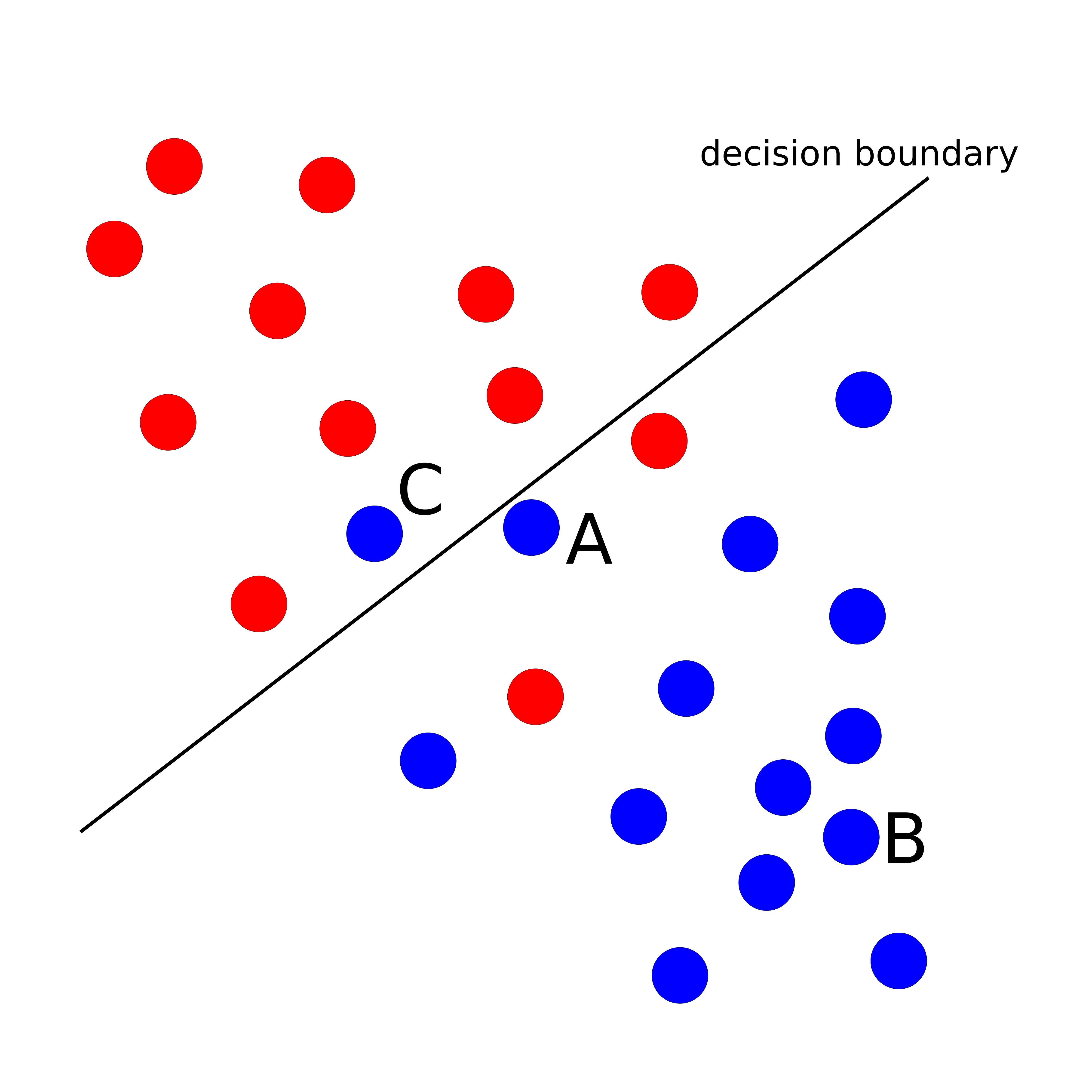
The goal of logistic regression is to identify a plane that maximizes the distance between instances of one class and the decision boundary, in the appropriate direction.

Logistic Regression widget in Orange offers the advantage of interpretability through the use of a Nomogram.

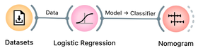
A nomogram displays the relative importance of variables in a model. The importance of a variable is indicated by its position on the nomogram: variables higher up on the list are more important. In addition, the length of the line corresponding to each variable indicates its relative importance: longer lines indicate more important variables. Each line represents the coefficient of the corresponding variable, which is used to compute the probability of the target class. By adjusting the blue point along a line, you can explore how changing the value of the corresponding variable affects the model's output, demonstrating the relationship between different input values and the predicted probability of the target class.

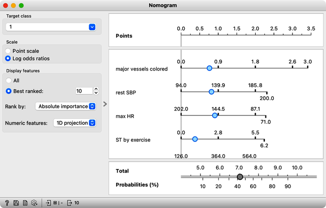
Logistic regression takes into account the correlation among variables when evaluating them simultaneously. In cases where some variables are correlated, their importance is distributed among them.

However, logistic regression has limitations as it relies on linear decision boundaries, which means that it may not work well for datasets that cannot be separated in this way. Can you think of an example of such a dataset?

Chapter 5: Random Forest

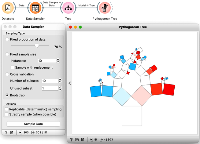
The random forest algorithm develops each tree on a bootstrap sample, which is a sample with the same number of instances as the original dataset. In a bootstrap sample, each data instance is drawn from the original dataset with replacement, creating a new dataset that includes approximately 63% of the original samples. The remaining 37% of the data instances can be used to estimate accuracy and feature importance.

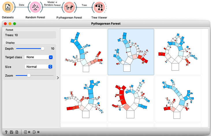
Random forests, a modeling technique introduced in 2001, remains one of the most effective classification and regression methods. Unlike traditional decision trees that choose the feature with the best separation at each node, random forests build multiple trees using a random selection of features and data samples. This approach introduces variability in the tree-building process and can improve model performance. By randomly selecting among best-ranked features at each node, the models can account for interactions among variables and prevent overfitting. One way to visualize the impact of random sampling on tree structure is to use a tree visualization widget like Pythagorean Tree. By sampling the data with each tree construction, the resulting trees can vary substantially, allowing for greater model flexibility and robustness. We demonstrate this approach using a heart disease dataset.

Random forest trees are generally quite diverse, and for the final prediction, the trees collectively "vote" for the best class. This voting process is similar to asking a group of people with varying levels of expertise to make a decision by majority vote. While some people may not have enough knowledge to make an informed decision and will vote randomly, others may have relevant knowledge that will influence the decision in the correct direction. By aggregating the results of many trees, random forests can incorporate the knowledge of a diverse set of models to make accurate predictions.

Interpreting a random forest model can be challenging due to the many tree models involved. Understanding which features are the most important in a random forest can be particularly challenging. Fortunately, the creators of random forests have defined a procedure for computing feature importances. This importance is assessed by measuring the accuracy of each tree on its out-of-sample testing data when the tree uses the original testing data or the data with shuffled values of a chosen feature. Features that have a large difference in accuracy are deemed more important. To obtain this ranking, one can use a Random Forest learner with a Rank widget. This approach can help users identify the most important features and understand how they contribute to the model's predictions.

Why do you think Random Forest does not need a connection from Datasets in the workflow on the right?

It is advantageous to compare the accuracy of random forests to that of classification trees. In practical applications, random forests consistently outperform classification trees in terms of precision and achieve higher classification accuracy.