Tuesday: Classification

Chapter 1: Image Embedding

Every dataset we have encountered so far has been in matrix (tabular) form, where objects—such as tissue samples, students, or flowers—are described by row vectors representing a set of features. However, not all data naturally fits this format. Consider collections of text articles, nucleotide sequences, voice recordings, or images. Ideally, we would transform these types of data into the same matrix format we have used so far. This would allow us to represent collections of images as matrices and analyze them using familiar prediction and clustering techniques.

Until recently, finding a useful representation of complex objects such as images was a challenging task. Now, deep learning enables the development of models that transform complex objects into numerical vectors. While training such models is computationally demanding and requires large datasets, we can leverage pre-trained models to efficiently represent our data as numerical features.

Consider images. When we, as humans, perceive an image, we process information hierarchically—starting from pixels, then recognizing spots and patches, and eventually identifying higher-order structures** such as squares, triangles, and frames, leading to the recognition of complex objects. Artificial neural networks in deep learning emulate this process through layers of computational units, which function as logistic regression models enhanced with additional mechanisms, such as computing weighted sums, maximums, or selectively processing subsets of input data—details we will not cover here.

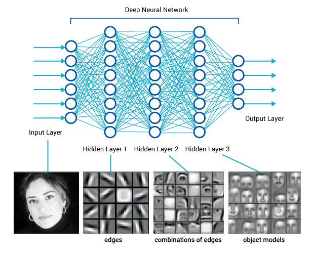
If we feed an image into such a network and extract the outputs from the deeper layers—typically from the penultimate layer—we obtain a vector that represents the image and encodes its semantics. This vector contains numerical values that, ideally, capture information about higher-order shapes or even objects within the image. While this representation is not necessarily interpretable in a human-understandable way, it is still valuable, as it encodes meaningful features. Using this representation, we can apply unsupervised or supervised machine learning techniques to images, enabling the discovery of groups with shared semantics.

The process of representing images as numerical vectors, as described above, is called embedding. Let's now demonstrate how to apply this technique in Orange. We will begin with the following workflow.

Download the zipped file with sketches of animals and load it in Orange using Import Images widget.

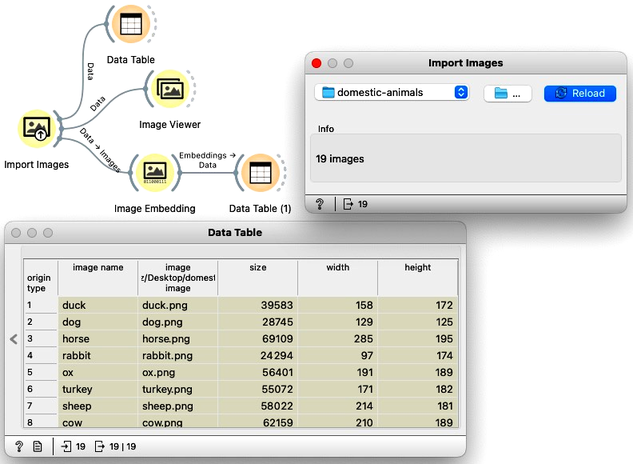
In the workflow, we first load the images from a directory and inspect the data. The Data Table reveals that Orange primarily stores the file locations and sizes, but no meaningful features are available yet. To visualize the images listed in the data table, we use the Image Viewer. This step is useful to verify that the directory structure has been read correctly and that all intended images are included in the analysis.

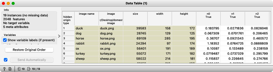
The most important part of our workflow is the embedding step. Deep learning requires a large amount of data (thousands to millions of instances) and significant computational power to train a network. Instead of training a new model, we use a pre-trained one. Even so, the embedding process takes time, so Orange does not perform it locally but instead uses a server accessed through the Image Embedding widget. This step converts images into a set of 2048 numerical features, which are then appended to the table alongside the image meta-features.

Embedding results in images described by thousands of features. Due to the curse of dimensionality, Euclidean distance becomes ineffective: in high-dimensional spaces, distances between points tend to concentrate, making all images appear similarly distant from one another. This phenomenon arises because, as the number of dimensions increases, the absolute difference between distances shrinks, reducing the discriminatory power of Euclidean distance. As a result, finding truly "similar" images using Euclidean distance becomes unreliable. A more appropriate measure is cosine distance, which considers the angle between high-dimensional vectors rather than their absolute magnitude. Cosine distance captures similarity based on direction, making it more robust for high-dimensional embeddings where magnitude differences may not be meaningful. This is particularly useful for deep learning embeddings, where the feature space often encodes semantic similarity more effectively in terms of orientation rather than strict spatial proximity.

We have no clear understanding of what these features represent, except that they capture higher-level abstract concepts within the deep neural network (which, admittedly, is not very helpful for interpretation). However, we have successfully transformed images into numerical vectors, allowing us to compare them and measure their similarities and distances. Distances? Right, we can use them for clustering. Let's cluster the images of animals and see what happens.

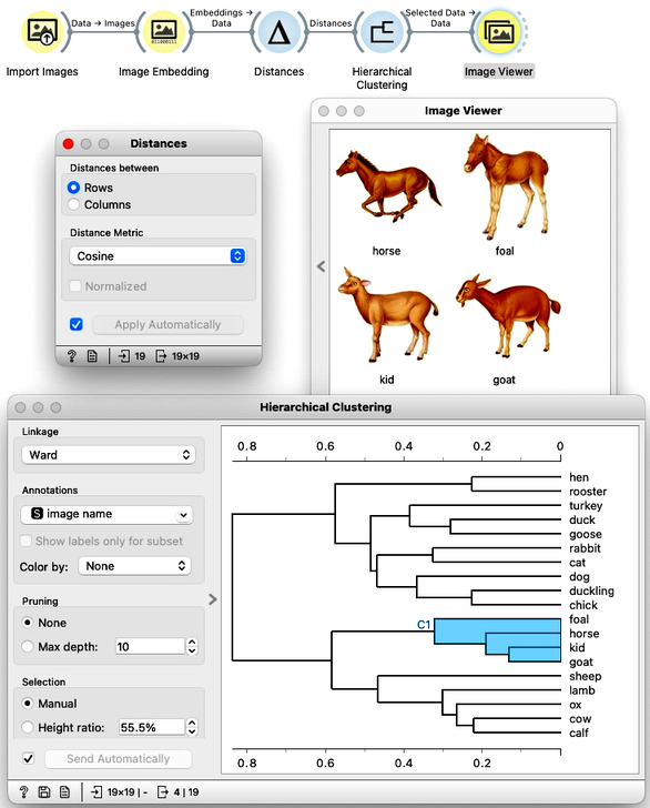
To recap: In the workflow above, we loaded the images from the local disk, converted them into numerical representations, computed a distance matrix containing distances between all pairs of images, performed hierarchical clustering using these distances, and displayed the images corresponding to a selected branch of the dendrogram in the Image Viewer. We used cosine similarity to measure distances, as it produced a more meaningful dendrogram compared to Euclidean distance.

At this stage, we now understand how to convert images into useful numerical vectors—a process known as embedding. This representation allows us to apply various analytical techniques, including clustering, PCA, t-SNE visualizations of image maps, classification, and regression. Rather than detailing all these applications here, we refer the reader to an article on image analytics with Orange and invite them to watch the following set of videos, which further explain image classification and retrieval of similar images using Orange.

These videos are somewhat dated, and some of the widgets used in them may have been redesigned. However, the concepts they illustrate remain the same, as do most, if not all, of the widget names.

Chapter 2: Classification

We call the variable we wish to predict a target variable, or an outcome or, in traditional machine learning terminology, a class. Hence we talk about classification, classifiers, classification trees...

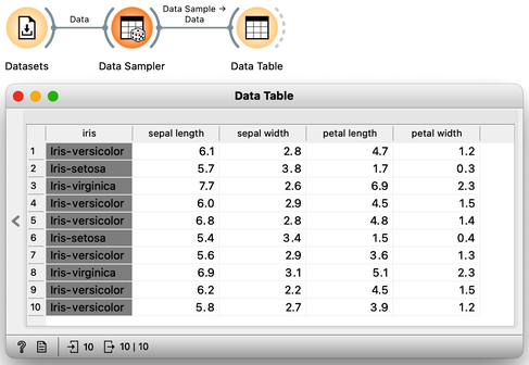
The Iris data set 150 Iris flowers, each of which can be distinguished based on the width and length of their sepals and petals. Although it may be challenging for an untrained observer to differentiate between the different types of Iris flowers, the data set, which dates back to 1936, actually includes three distinct species - Iris setosa, Iris versicolor, and Iris virginica - with 50 flowers belonging to each species. To access the Iris data, one can utilize the Datasets widget. Presented below is a small excerpt of the Iris data set:

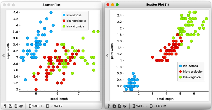
Let's examine the Iris flower data using a scatterplot, with two distinct projections. It's evident that the combination of petal and leaf measurements creates a clearer separation of the three classes. This separation is so distinct that we could potentially use a set of rules based on the two measurements to predict the species of Iris.

Speaking of prediction, classifying the flowers into one of the three species is precisely what we want to accomplish. Imagine visiting a flower shop, taking the flower's measurements, and then using them to determine its species. This would be an impressive feat, transforming even regular customers into knowledgeable botanists.

A model that uses the morphological characteristics of the Iris, such as sepal and petal measurements, to classify the species of Iris is known as a classification model. The Iris flowers in our data set are classified into one of the three distinct categories, and the task at hand is classification.

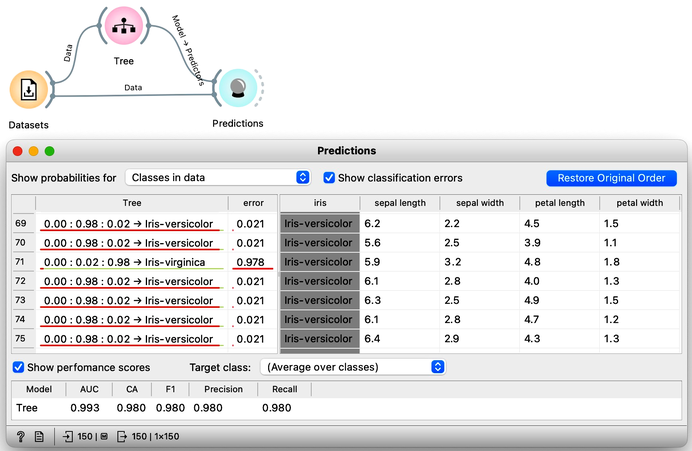
To create a classification model, we feed the data into the Tree widget, which then infers a classification model and transfers it to the Predictions widget. Unlike previous workflows where the widgets mostly communicated passed data tables to each other, there is now a channel that carries a predictive model. The Predictions widget also receives the data from the Datasets widget and uses the model on its input to make predictions about the data, which are then displayed in a table in the "Tree" column. Visible are also inferred probabilities of each of the three classes.

Something in this workflow is conceptually wrong. Can you guess what?

How correct are these predictions? Do we have a good model? How can we tell? But (and even before answering these very important questions), what is a classification tree? And how does Orange create one? Is this algorithm something we should really use? So many questions to answer.

Chapter 3: Trees

Classification trees were hugely popular in the early years of machine learning, when they were first independently proposed by the engineer Ross Quinlan (C4.5) and a group of statisticians (CART), including the father of random forests Leo Brieman.

In the previous lesson, we used a classification tree, one of the oldest, but still popular, machine learning methods. We like it since the method is easy to explain and gives rise to random forests, one of the most accurate machine learning techniques (more on this later). What kind of model is a classification tree?

Let us load the iris flowers data set, build a classification tree using the Tree widget and visualize it in a Tree Viewer.

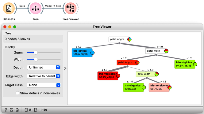
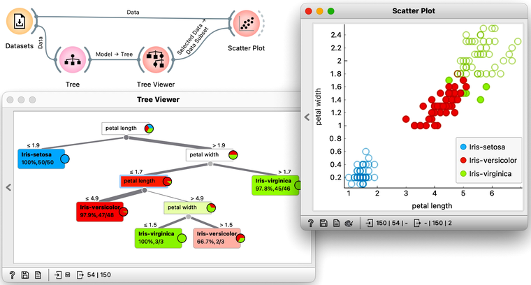
We read the tree from top to bottom. Looks like the feature "petal length" best separates the iris species setosa from the others, and in the next step, "petal width" then almost perfectly separates the remaining two species.

Trees place the most useful feature at the root. What would be the most useful feature? The feature that splits the data into two purest possible subsets. It then splits both subsets further, again by their most useful features, and keeps doing so until it reaches subsets in which all data belongs to the same class (leaf nodes in strong blue or red) or until it runs out of data instances to split or out of useful features (the two leaf nodes in white).

The Rank widget can be used on its own to show the best predicting features. Say, to figure out which genes are best predictors of the phenotype in some gene expression data set, or to infer what socioeconomic feature is most related to country's well-being.

We still have not been very explicit about what we mean by "the most useful" feature. There are many ways to measure the quality of features, based on how well they distinguish between classes. We will illustrate the general idea with information gain. We can compute this measure in Orange using the Rank widget, which estimates the quality of data features and ranks them according to how informative they are about the class. We can either estimate the information gain from the whole data set, or compute it on data corresponding to an internal node of the classification tree in the Tree Viewer.

The following example uses the Sailing data set, which includes three features and a class. The data set observes, say, a friend who likes to sail. Suppose that every Wednesday, we ask her what kind of boat she has available and the size of the company that will join her, look at the weather forecast, and then record if she went sailing during the weekend. In the future, we are intrigued to predict on Wednesday if she will go sailing. We would also like to know which of the three features bears the most information about the prediction. Here is the workflow where we use the Rank widget on the whole data set and the data sets that are intrinsic to every note of the classification tree to check if the chosen variable in that node is indeed the most informative one.

Try to assemble this workflow, open the widgets, and select any of the internal nodes of the tree from the Tree Viewer. Check out the resulting changes in the Rank (1) and Data Table (1).

Besides the information gain, the Rank widget displays several other measures, including Gain Ratio and Gini index, which are often quite in agreement and were invented to better handle discrete features with many different values.

Note that the Data widget needs to be connected to the Scatter Plot's Data input and Tree Viewer to the Scatter Plot's Data Subset input. Do this by connecting the Data and Scatter Plot first.

To explore the tree model further, here is an interesting combination of a Tree Viewer and a Scatter Plot. This time, we will again use the Iris flower data set. In the Scatter Plot, we can first find the best visualization of this data set, the one that best separates the instances from different classes. Then we connect the Tree Viewer to the Scatter Plot. Data instances from the selected node of the Tree Viewer, flowers that satisfy the criteria that lead to that node, are highlighted in the Scatter Plot.

We could include a few other widgets in this workflow for fun. Say, connecting the Tree Viewer with a Data Table and Distributions widget. Or connecting it to a Box Plot, but then rewiring the connection to pass all the data to it and sub-grouping the visualization by a feature called "Selected". Like below.

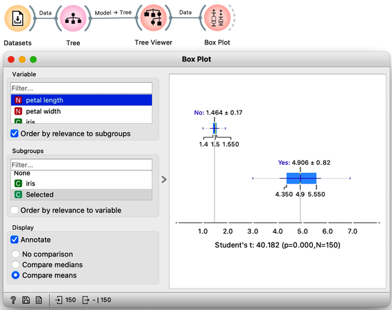
In a way, a Tree Viewer behaves like Select Rows, except that the rules used to filter the data are inferred from the data itself and optimized to obtain purer data subsets.