Data Mining @ BCM

Chapter 1: Image Embedding

Every dataset we have encountered so far has been in matrix (tabular) form, where objects—such as tissue samples, students, or flowers—are described by row vectors representing a set of features. However, not all data naturally fits this format. Consider collections of text articles, nucleotide sequences, voice recordings, or images. Ideally, we would transform these types of data into the same matrix format we have used so far. This would allow us to represent collections of images as matrices and analyze them using familiar prediction and clustering techniques.

Until recently, finding a useful representation of complex objects such as images was a challenging task. Now, deep learning enables the development of models that transform complex objects into numerical vectors. While training such models is computationally demanding and requires large datasets, we can leverage pre-trained models to efficiently represent our data as numerical features.

Consider images. When we, as humans, perceive an image, we process information hierarchically—starting from pixels, then recognizing spots and patches, and eventually identifying higher-order structures** such as squares, triangles, and frames, leading to the recognition of complex objects. Artificial neural networks in deep learning emulate this process through layers of computational units, which function as logistic regression models enhanced with additional mechanisms, such as computing weighted sums, maximums, or selectively processing subsets of input data—details we will not cover here.

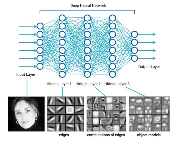
If we feed an image into such a network and extract the outputs from the deeper layers—typically from the penultimate layer—we obtain a vector that represents the image and encodes its semantics. This vector contains numerical values that, ideally, capture information about higher-order shapes or even objects within the image. While this representation is not necessarily interpretable in a human-understandable way, it is still valuable, as it encodes meaningful features. Using this representation, we can apply unsupervised or supervised machine learning techniques to images, enabling the discovery of groups with shared semantics.

The process of representing images as numerical vectors, as described above, is called embedding. Let's now demonstrate how to apply this technique in Orange. We will begin with the following workflow.

Download the zipped file with sketches of animals and load it in Orange using Import Images widget.

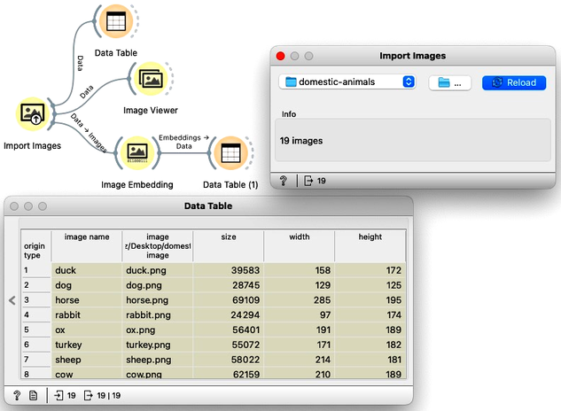
In the workflow, we first load the images from a directory and inspect the data. The Data Table reveals that Orange primarily stores the file locations and sizes, but no meaningful features are available yet. To visualize the images listed in the data table, we use the Image Viewer. This step is useful to verify that the directory structure has been read correctly and that all intended images are included in the analysis.

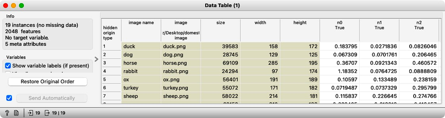
The most important part of our workflow is the embedding step. Deep learning requires a large amount of data (thousands to millions of instances) and significant computational power to train a network. Instead of training a new model, we use a pre-trained one. Even so, the embedding process takes time, so Orange does not perform it locally but instead uses a server accessed through the Image Embedding widget. This step converts images into a set of 2048 numerical features, which are then appended to the table alongside the image meta-features.

Embedding results in images described by thousands of features. Due to the curse of dimensionality, Euclidean distance becomes ineffective: in high-dimensional spaces, distances between points tend to concentrate, making all images appear similarly distant from one another. This phenomenon arises because, as the number of dimensions increases, the absolute difference between distances shrinks, reducing the discriminatory power of Euclidean distance. As a result, finding truly "similar" images using Euclidean distance becomes unreliable. A more appropriate measure is cosine distance, which considers the angle between high-dimensional vectors rather than their absolute magnitude. Cosine distance captures similarity based on direction, making it more robust for high-dimensional embeddings where magnitude differences may not be meaningful. This is particularly useful for deep learning embeddings, where the feature space often encodes semantic similarity more effectively in terms of orientation rather than strict spatial proximity.

We have no clear understanding of what these features represent, except that they capture higher-level abstract concepts within the deep neural network (which, admittedly, is not very helpful for interpretation). However, we have successfully transformed images into numerical vectors, allowing us to compare them and measure their similarities and distances. Distances? Right, we can use them for clustering. Let's cluster the images of animals and see what happens.

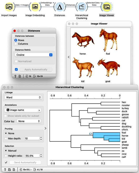
To recap: In the workflow above, we loaded the images from the local disk, converted them into numerical representations, computed a distance matrix containing distances between all pairs of images, performed hierarchical clustering using these distances, and displayed the images corresponding to a selected branch of the dendrogram in the Image Viewer. We used cosine similarity to measure distances, as it produced a more meaningful dendrogram compared to Euclidean distance.

At this stage, we now understand how to convert images into useful numerical vectors—a process known as embedding. This representation allows us to apply various analytical techniques, including clustering, PCA, t-SNE visualizations of image maps, classification, and regression. Rather than detailing all these applications here, we refer the reader to an article on image analytics with Orange and invite them to watch the following set of videos, which further explain image classification and retrieval of similar images using Orange.

These videos are somewhat dated, and some of the widgets used in them may have been redesigned. However, the concepts they illustrate remain the same, as do most, if not all, of the widget names.