Data Mining @ BCM

Chapter 1: Linear Regression

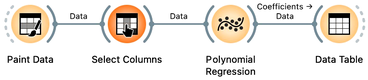
For a start, let us construct a very simple data set. It will contain just one continuous input feature (let's call it x) and a continuous class (let's call it y). We will use Paint Data, and then reassign one of the features to be a class using Select Columns widget, moving the feature y from "Features" to "Target Variable". It is always good to check the results, so we are including Data Table and Scatter Plot in the workflow at this stage. We will be modest this time and only paint 10 points and use Put instead of the Brush tool.

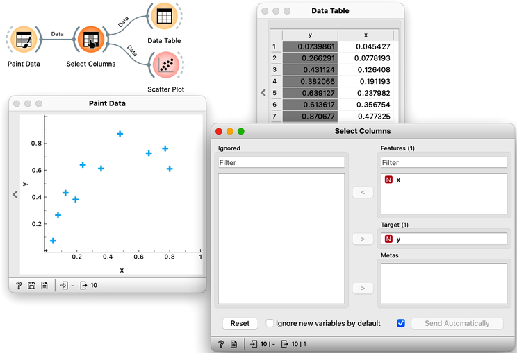
We want to build a model that predicts the value of the target variable y from the feature x. Say that we would like our model to be linear, to mathematically express it as $h(x)=w_0+w_1 x$. Oh, this is the equation of a line. So we would like to draw a line through our data points. The w0 is then an intercept, and $w_1$ is a slope. But there are many different lines we could draw. Which one is the best? Which one is the one that fits our data the most? Are they the same?

Do not worry about the strange name of the Polynomial Regression, we will get there in a moment.

The question above requires us to define what a good fit is. Say, this could be the error the fitted model (the line) makes when it predicts the value of $y$ for a given data point (value of $x$). The prediction is $h(x)$, so the error is $h(x) - y$. We should treat the negative and positive errors equally, plus — let us agree — we would prefer punishing larger errors more severely than smaller ones. Therefore, we should square the errors for each data point and sum them up. We got our objective function! It turns out that there is only one line that minimizes this function. The procedure that finds it is called linear regression. For cases where we have only one input feature, Orange has a special widget in the Educational add-on called Polynomial Regression.

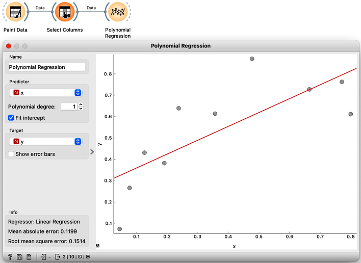Looks ok, except that these data points do not appear exactly on the line. We could say that the linear model is perhaps too simple for our data set. Here is a trick: besides the column $x$, the widget Polynomial Regression can add columns $x^2$, $x^3$, …, $x^n$ to our data set. The number $n$ is a degree of polynomial expansion the widget performs. Try setting this number to higher values, say to 2, and then 3, and then, say, to 8. With the degree of 3, we are then fitting the data to a linear function $h(x) = w_0 + w_1 x + w_2 x^2 + w_3 x^3$. Note that $x^k$, that is, the powers of $x$ are just new features, and our model $h(x)$ is still a linear combination of features and weights.

The trick we have just performed is polynomial regression, adding higher-order features to the data table and then performing linear regression. Hence the name of the widget. We get something reasonable with polynomials of degree 2 or 3, but then the results get wild. With higher degree polynomials, we overfit our data.

It is quite surprising to see that the linear regression model can fit non-linear (univariate) functions. It can fit the data with curves, such as those on the figures. How is this possible? Notice, though, that the model is a hyperplane (a flat surface) in the space of many features (columns) that are the powers of $x$. So for the degree 2, $h(x)=w_0 + w_1 x + w_2 x^2$ is a (flat) hyperplane. The visualization gets curvy only once we plot $h(x)$ as a function of $x$.

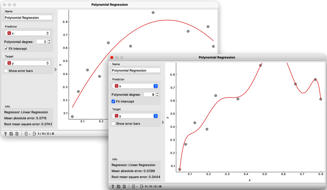
Overfitting is related to the complexity of the model. In polynomial regression, the parameters w define the model. With the increased number of parameters, the model complexity increases. The simplest model has just one parameter (an intercept), ordinary linear regression has two (an intercept and a slope), and polynomial regression models have as many parameters as the polynomial degree. It is easier to overfit the data with a more complex model, as it can better adjust to the data. But is the overfitted model discovering the true data patterns? Which of the two models depicted in the figures above would you trust more?

Chapter 2: Regularization

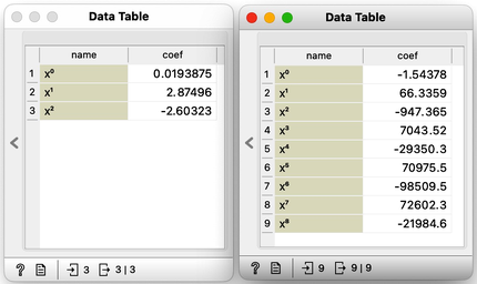
There has to be some cure for overfitting. Something that helps us control it. To find it, let's check the values of the parameters "w" under different degrees of polynomials.

With smaller degree polynomials, values of feature weights stay small, but then as the degree goes up, the numbers get huge.

Which inference of linear model would overfit more, the one with high or with low regularization strength? What should the value of regularization strength be to cancel regularization? What if regularization strength is high, say 1000?

More complex models have the potential to fit the training data better, but they often produce a fitted curve that wiggles sharply. Since the derivatives of such functions are high, the coefficients "w" must also be high. However, it is possible to encourage linear regression to infer models with small coefficients. We can modify the optimization function that linear regression minimizes, which is the sum of squared errors. By adding a sum of all "w" squared to this function and asking linear regression to minimize both terms, we can achieve regularization. We may also weigh the "w" squared part with a coefficient, such as "w," to control the level of regularization.

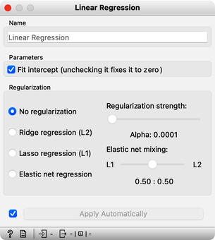
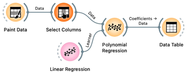
Here we go: we just reinvented regularization, which helps machine learning models not to overfit the training data. To observe the effects of regularization, we can give Polynomial Regression to our linear regression learner, which supports these settings.

Internally, if no learner is present on its input, the Polynomial Regression widget would use just ordinary, non-regularized linear regression.

The Linear Regression widget offers two types of regularization techniques. Ridge regression, which we previously discussed, minimizes the sum of squared coefficients "w." In contrast, Lasso regression minimizes the sum of the absolute value of coefficients. While the difference may appear minor, Lasso regression can lead to a significant portion of coefficients "w" becoming zero, effectively performing feature subset selection.

Let's move on to the test. Set the degree of polynomial to the maximum and apply Ridge Regression. Does the inferred model overfit the data? How does the degree of overfitting vary with changes in regularization strength?

Chapter 3: Accuracy

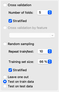
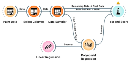
Paint about 20 to 30 data instances. Use the attribute y as the target variable in Select Columns. Split the data 50:50 in Data Sampler. Cycle between "Test on train data" and "Test on test data" in Test and Score. Use ridge regression to build a linear regression model.

Overfitting hurts. Overfit models fit the training data well but can perform miserably on new data. Let us observe this effect in regression. We will use hand-painted data set, split it into the training (50) and test (50) data set, polynomially expand the training data set to enable overfitting and build a model. We will test the model on the already seen training data and the unseen held-out data.

Now we can vary the regularization strength in Linear Regression and observe the accuracy in Test and Score. For accuracy scoring, we will use RMSE, root mean squared error, which is computed by observing the error for each data point, squaring it, averaging this across all the data instances, and taking a square root.

The core of this lesson is to compare the error on the training and test set while varying the level of regularization. Remember that regularization controls overfitting. The more we regularize, the less tightly we fit the model to the training data. So for the training set, we expect the error to drop with less regularization and more overfitting. The error on the training data increases with more regularization and less fitting. We expect no surprises here. But how does this play out on the test set? Which sides minimizes the test-set error? Or is the optimal level of regularization somewhere in between? How do we estimate this level of regularization from the training data alone?

Orange is currently not equipped with the fitting of meta parameters, like the degree of regularization, and we need to find their optimal values manually. At this stage, it suffices to say that we must infer meta parameters from the training data set without touching the test data. If the training data set is sufficiently large, we can split it into a set for training the model and a data set for validation. Again, Orange does not support such optimization yet, but it will sometime in the future. :)

Chapter 4: Live Long

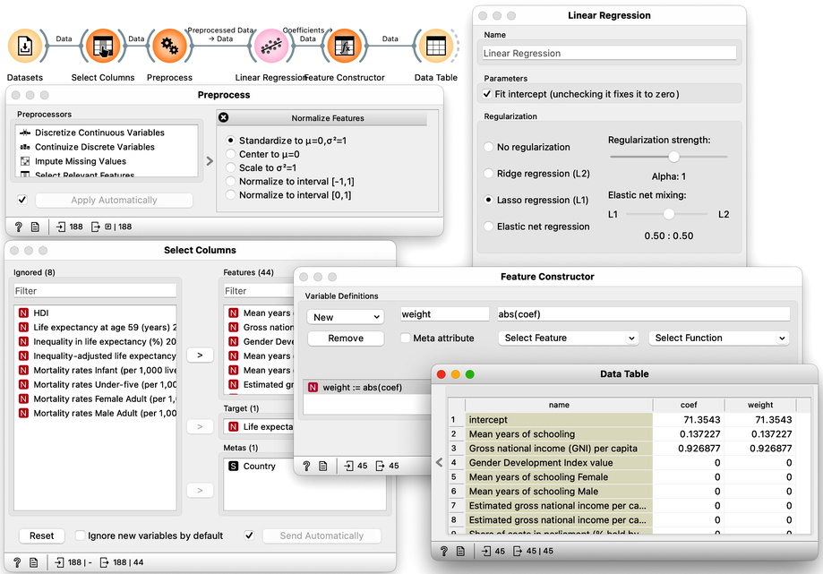
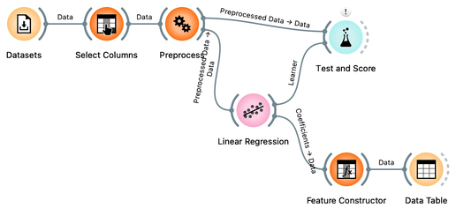
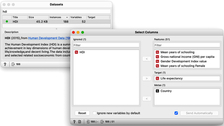
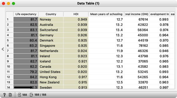
Previously, we demonstrated the pitfalls of overfitting by applying linear regression to a painted dataset. In this exercise, we will apply regression modeling to real data and utilize the tools we have learned so far. Specifically, we will use socioeconomic data from the HDI dataset explored in prior lectures to predict a country's average life expectancy. Our objectives are twofold: first, to evaluate the predictive accuracy of the resulting model, and second, to identify which factors have the strongest correlation with life expectancy and are therefore critical in the predictive model. Here is our workflow:

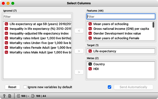
We start with defining the initial structure of the data set. Original data has no target. We are using Select Columns widget, move the "Life Expectancy" to the Target box. That is it for now. Later, Select Columns will become useful to remove some of the variables that are a tautology to life expectancy, and some of the variables that are perhaps too obviously related to life expectancy and which we would not like to appear in our model.

One of our goals is to evaluate the influence of different features in the linear model. Linear models are comprised of weighted sums of input features, and the weights can provide insight into the significance of each feature in the model. However, to accurately determine importance, we must consider the varying ranges of feature values in our dataset. For example, years of schooling may range from 2 to 15, while gross national income per capita may range from a thousand to 140 thousand.

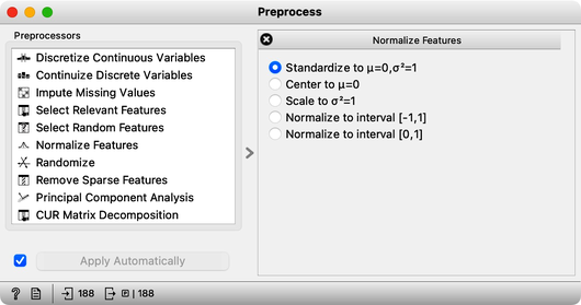
If both features were equally important in predicting life expectancy, the weight of the schooling feature in the model would be much larger than that of income simply because income is expressed in higher numbers. To accurately compare weights, we must standardize the range of values for each variable. We can do this using the Preprocess widget, which standardizes the data.

At this stage, it's always helpful to take a closer look at the data to ensure that our model is behaving as expected. One way to do this is by using the Connect Data Table widget to examine the output of the Preprocess widget and verify that the data has been properly standardized. Additionally, we can use tools such as Box Plot or Distributions to further visualize the impact of standardization on the data and confirm that it aligns with our expectations. By closely inspecting the data, we can ensure that our model is based on accurate and reliable information, and that our results are meaningful and trustworthy.

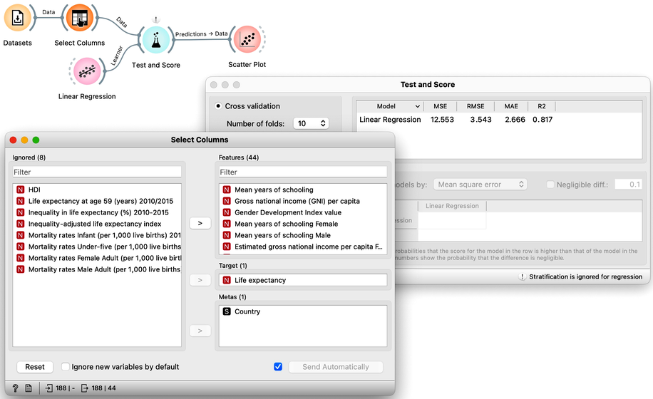
We are now ready to check cross-validated performance of our model.

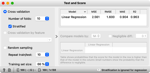
Great, it looks like our model is performing well! On average, our predictions are only off by 1.6 years. We can see this by looking at the root mean squared error (RMSE), which is a useful measure of the overall error in our model. However, it's important to note that the value of RMSE can be influenced by the distribution of our target variable. In this case, since average life expectancy ranges from about 50 to 90, an RMSE of 1.6 seems quite small, which suggests that our model is of high quality. Overall, we can be confident that, with current selection of the features and considering the accuracy alone, our model is accurately predicting life expectancy.

There is another measure that we have available and for which we do not have to know about the distribution of the target variable. The coefficient of determination (R2). In essence, R2 compares the squared error between our model and the uninformed model which predicts with the mean of the target variable in the training set. It computes the ration of these two errors. If our model predicts well, the ratio approaches 0, and if it predicts badly than its predictions are similar to those of the mean and hence the ratio is 1. Since we prefer a better score for a better model, R2 reports on 1 minus our ratio. That is, R-squared ranges between 0 and 1, with a value of 0 indicating that the model explains none of the variation in the dependent variable and a value of 1 indicating that the model explains all of the variation in the dependent variable. However, it is rare to achieve an R-squared value of 1.

Our R2 at this stage is 0.963. This looks too good to be true. It is time to look at our model, that is, its weights. We feed the data to the Linear Regression, and hence use the same widget to deliver the learner for the Test and Score as well as the model trained on the entire Data. We could observe the coefficients of the model directly by feeding the output of the Linear Regression to the Data Table.

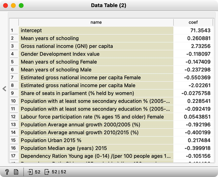
It's important to note that the weights assigned to features in our model can be either positive or negative, depending on the type of effect the features have on life expectancy. For example, mean years of schooling is positively related to life expectancy, while population annual growth has a negative effect. However, since we're interested in the overall effect of the features, rather than their specific direction, we should focus on the absolute values of the weights. To create such a feature, we can use the Feature Constructor widget, which can help us to better understand which features are having the greatest impact on the outcome of interest.

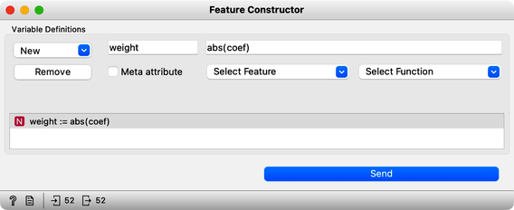
Now that we have computed the absolute weights, here they are:

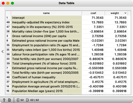
The intercept term in a model is a constant value that is added to the output, but it is not a weight that provides insights into the underlying factors affecting the outcome. Instead, we should focus on the other weights in the model, which can tell us which variables are important in determining the outcome. For example, if we are interested in predicting life expectancy, we would want to exclude features that report on adjusted life expectancy, as these variables are directly computed from average life expectancy. Similarly, including features that report on mortality statistics may not be informative, as their relationship with life expectancy is already well-established. By carefully selecting the variables in our model, we can improve our understanding of the factors that influence the outcome of interest.

In order to refine our model, we can iteratively remove features that we would like to exclude using the "Select Columns" method, check the weights, and observe the resulting estimated accuracy. Through this process, we aim to retain a model that is both accurate and interpretable, increasing our insight into its underlying structure. By carefully selecting which features to include, we can create a more streamlined and focused model that provides more valuable insights into the relationships between the variables of interest.

Chapter 5: Accuracy Analysis

The last lessons quickly introduced scoring for regression and essential measures such as RMSE and R2. In classification, the confusion matrix was an excellent addition to finding misclassified data instances. But the confusion matrix could only be applied to discrete classes. Before Orange gets some similar widgets for regression, one way to find misclassified data instances is through scatter plot. Let us demonstrate this on the regression model we have been developing on socioeconomic data, that is, on the HDI data set.

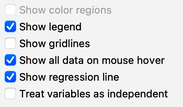
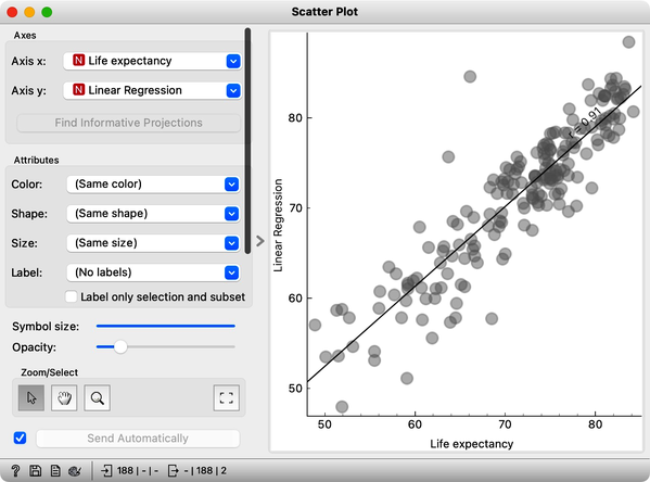
For the visualization on the right, we have switched on the option to show regression line between. This also informs us about correlation between the two variables, which is quite high at 0.91.

We would like to observe the cross-validated error of linear regression, or better, the correspondence between true class values and the predictions, when these were made when the data instance was in the training set. We use linear regression with L2 regularization, and in this example set the regularization strength to $\alpha=0.1$. In scatterplot, we plot the predicted value vs. the true class, and can note nice correspondence between the two.

Let us change this workflow to observe the absolute error of our prediction. Here is our workflow.

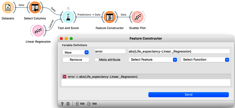
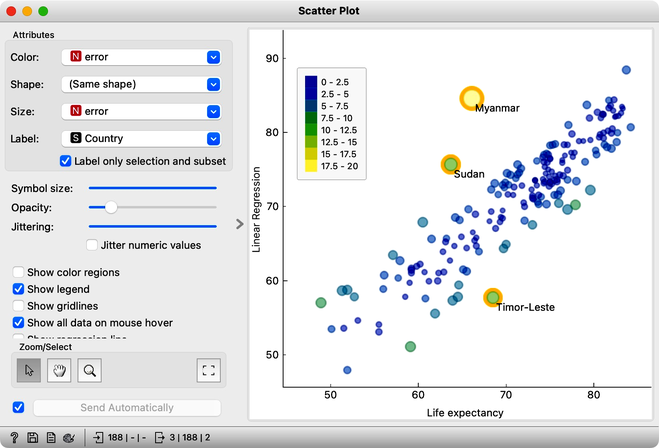
We used a Feature Constructor widget to compute the error. In scatterplot, we can set the plotting parameters so that we can expose the countries with largest prediction errors, and select them to plot their names.

Alternatively we could also sent the output of Feature Constructor to the Data Table, sort the countries according to the absolute prediction error, select those with the largest error and send them as a data subset to the Scatter Plot. Or use the Distributions widget for the similar task. We do not show these workflows here, as it is time for an engaged reader to experiment with these and other ideas.

Chapter 6: L1 and L2 Regularization

Regularization is a technique used in linear regression to prevent overfitting. During inference, the weights of the linear model are set to minimize the squared error on the training set. However, we also want to avoid models that are too complex or dynamic. To achieve this, we use normalization, which can be either L1 or L2. L2 regularization aims to minimize the sum of the squared feature weights, while L1 regularization sums their absolute values. Ridge regression refers to the inference of a linear model that includes L2 regularization, while lasso regression refers to the inference of a linear model that includes L1 regularization.

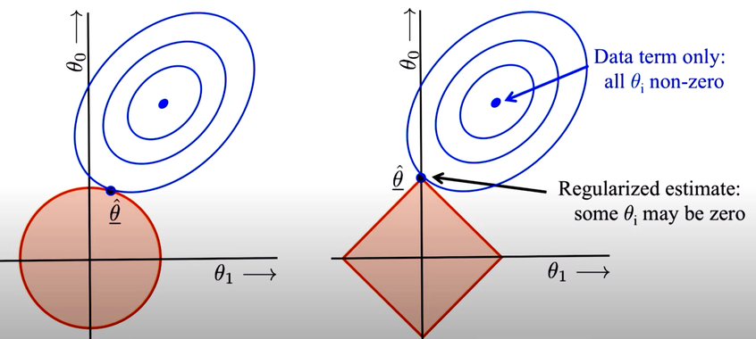
Although L1 and L2 regularization can result in similar models, they have different constraints. L2 regularization is roundish, while L1 regularization is squarish, with sharp corners and edges where some weights are 0. As a result, L1 regularization can lead to a linear model where some weights are 0, effectively excluding some features from the model. We can use L1 regularization for feature subset selection, which can help minimize the complexity of the model.

We have borrowed a conceptual graph from the web that illustrates the differences between two types of regularization: L1 and L2. While we won't delve deeply into the mathematical details (there are plenty of web pages and YouTube videos for this), we'll focus on practical applications and aim to explain the intuition behind L1 and L2 during our lectures. Our goal is to provide examples and real-world scenarios to help you understand how regularization can be used to improve machine learning models.

Let's conduct an experiment using the HDI dataset, which contains socio-economic data. We will normalize the features again to ensure that their weights are comparable, and pre-select relevant features for the model. We will then compare the results of using L1 and L2 regularization and observe how the ranked list of features changes. We will also investigate whether it's possible to obtain weights of exactly zero with L2 regularization and how changing the regularization strength parameter, $\alpha$, affects the results.